Introduction to Protection Relays 1

A fundamental aspect of understanding and effectively utilizing protection relays involves grasping the concept of Time Current Characteristic (TCC) curves. These curves, standardized under the International Electrotechnical Commission (IEC) standard 60255, are essential for the selection, coordination, and setting of protection relays in electrical networks.

Time Current Characteristic (TCC) Curves: The Basics

TCC curves graphically represent the relationship between the magnitude of the current flowing through the relay and the time it takes for the relay to operate. These curves are pivotal in designing and implementing protection schemes, as they enable engineers to determine how a relay will respond under different fault conditions. By analyzing TCC curves, engineers can ensure that relays operate accurately and selectively, clearing faults efficiently while minimizing the impact on the electrical system.

Comparing IEC 60255 Time Current Characteristic (TCC) Curves

Let us compare various TCC Curves of the Relay according to IEC 60255. These are all IDMT = Inverse Definite Minimum Time Relays. In this example, all the relays pickup (PMS = Plug Multiplier Setting) are at 0.95 full load current and all (TMS = Time Multiplier Setting) are set at 1.

Response to Overcurrents: SI, VI, and EI curves provide progressively faster responses to higher currents, with EI being the most responsive to high overcurrents. The variation in the steepness of these curves provides flexibility in coordinating devices in a power system network, allowing for selective tripping and minimizing disruption. Each curve type is tailored to specific system characteristics - SI for varying fault currents, VI for less variation, EI for minimal variation, LTI for overload conditions, and STI for quick response in complex coordination scenarios.

When comparing these curves, it's crucial to consider the specific requirements of the electrical system, including the nature of the load, the configuration of the network, and the expected range of fault conditions. The goal is always to ensure maximum protection with minimal disruption to the service.

Notice that their response curves "flatten out" beyond 20 times the full-load current of the equipment.

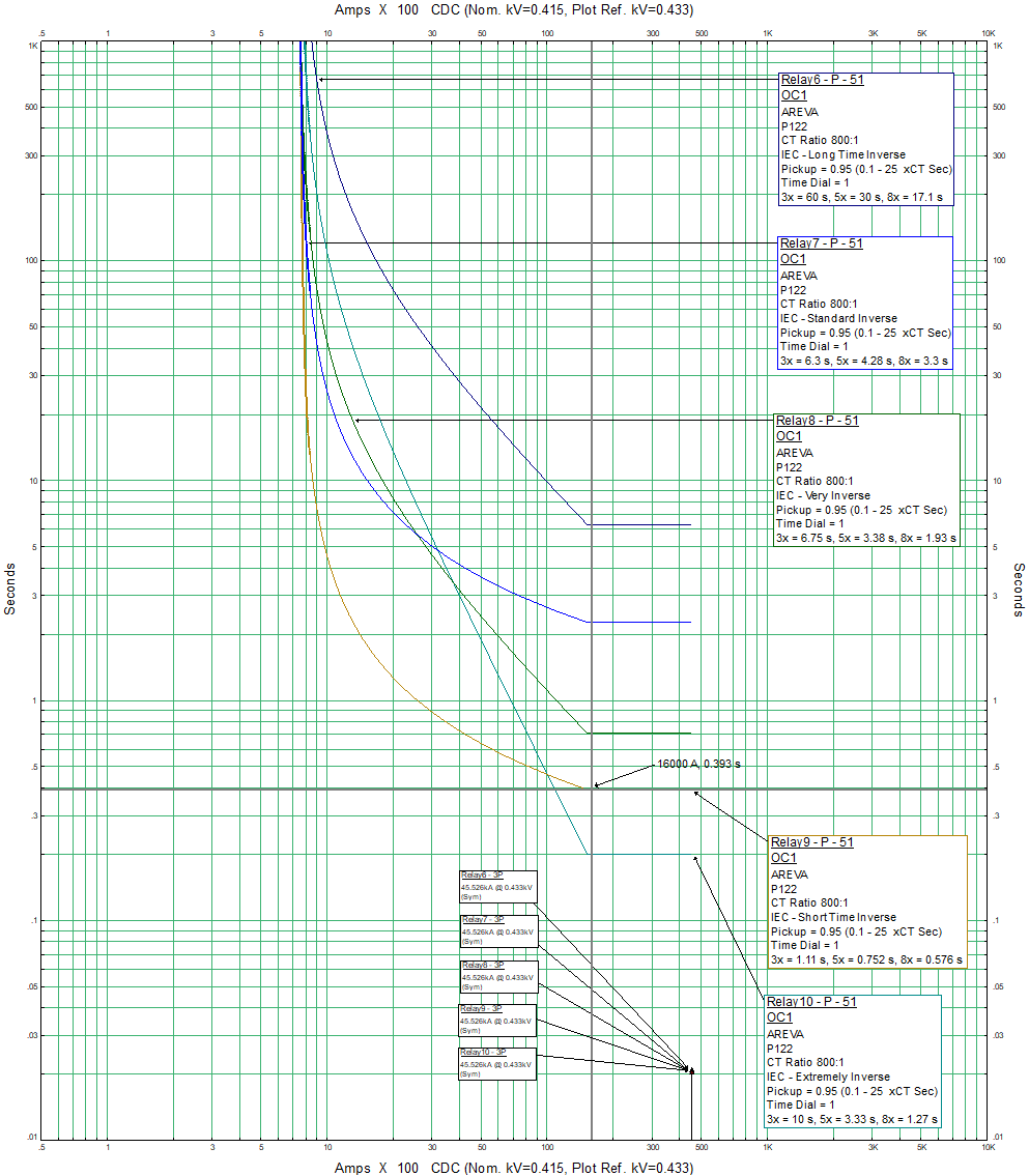
1. Standard Inverse (SI)

• Characteristic: The operating time decreases inversely with an increase in current.

• Application: Used where the fault current varies significantly with the location of the fault.

• Curve Shape: Moderately sloping; it provides a balance between speed and selectivity for a wide range of fault currents.

• IEC Equation:

  

  where T_MS​ is the time multiplier setting.

  

2. Very Inverse (VI)

• Characteristic: More inverse than Standard Inverse; the operating time decreases more steeply as the current increases.

• Application: Suitable for systems where fault currents do not vary significantly with distance, like in radial systems with significant impedance.

• Curve Shape: Steeper than SI, providing faster operation for higher currents.

• IEC Equation: Similar to SI but with different constants (A, α) providing a steeper curve.

  

3. Extremely Inverse (EI)

• Characteristic: Even more inverse than VI; the time decreases very steeply with increasing current.

• Application: Ideal for protecting long transmission lines where the fault current difference between the near-end and far-end faults is minimal.

• Curve Shape: Very steep, enabling quick response to high currents while allowing more time for lower-level faults.

• IEC Equation: Again, similar in form to SI and VI but with constants for an even steeper curve.

  

4. Long-Time Inverse (LTI)

• Characteristic: Has a much slower operation time compared to the SI characteristic.

• Application: Often used for overload protection rather than for fault conditions.

• Curve Shape: Much flatter, providing a longer delay, particularly suitable for overloads that are not immediately damaging.

• IEC Equation: Similar inverse relationship but with parameters set for much longer operating times.

  

5. Short-Time Inverse (STI)

• Characteristic: Designed for shorter operating times at higher currents.

• Application: Often used in coordination with other devices, allowing for brief overloads but protecting against sustained overcurrents.

• Curve Shape: Steeper than LTI, providing quick response to high overcurrents while allowing short-duration overloads.

• IEC Equation: Inverse curve with parameters set for shorter times.

  

When comparing these curves, it's crucial to consider the specific requirements of the electrical system, including the nature of the load, the configuration of the network, and the expected range of fault conditions. The goal is always to ensure maximum protection with minimal disruption to the service.

Join us on this electrifying journey and stay charged with "Engineer's Current"! 🌟🔌

🌟 Ignite Your Career with Engineer's Current! 🌟

Are you a young electrical engineer ready to power up your knowledge and career in the oil and gas industry? Don't miss out on "Engineer's Current" - your essential resource for in-depth insights, real-world case studies, and expert advice.

🔌 Subscribe Now and be part of an exclusive community where learning meets innovation. Stay ahead with the latest trends, deepen your expertise in electrical power systems, and connect with industry professionals.

💡 Take Charge of Your Future Today! Join "Engineer's Current" and turn your potential into high-voltage success!